Deephaven Quick Start Guide
The Quick Start Guide is designed to be a very short exercise to familiarize new users with the Deephaven interface, provide examples of using the Deephaven query language to generate tables and plots, save queries, and build a customized workspace.
Prerequisites
- Deephaven needs to be installed for your enterprise.
- The Deephaven Launcher application needs to be installed on your PC, with an instance configured to access the stored data.
Step 1 - Open Deephaven
When you first open Deephaven, you should see a screen similar to the one shown below.
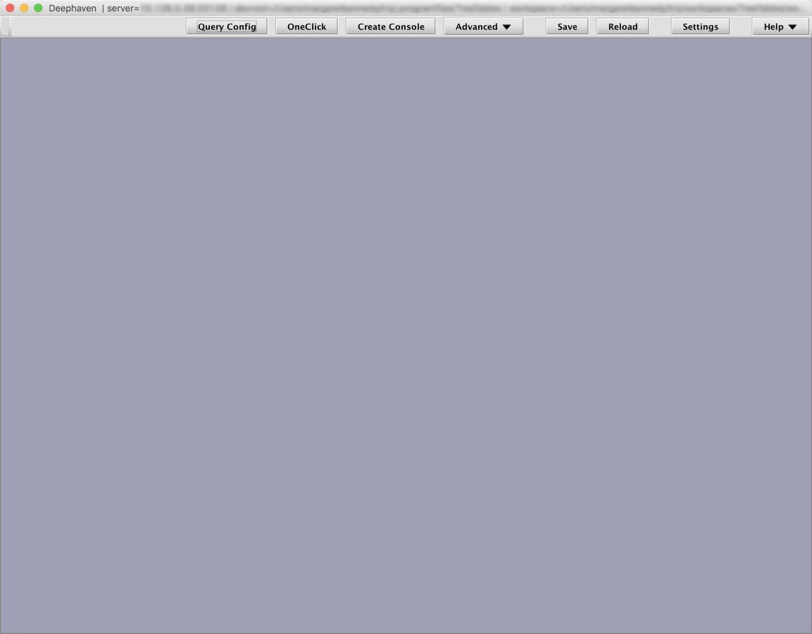
There is not much to see now, but this empty console window is the blank canvas you will ultimately use to create your own customized workspace.
Click the Create Console button at the top of the interface. A dialog window will then present an option to rename the panel.
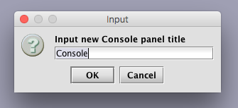
Click OK to keep the same name.
The interface will then change and present two new panels as shown below. 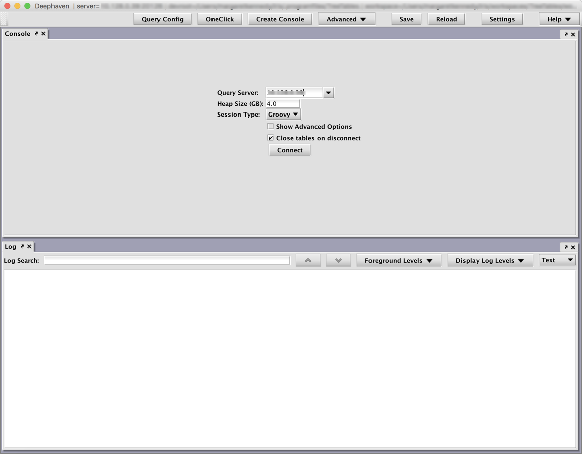
The Console panel at the top is used to enter your queries and run your analyses. The Log panel at the bottom presents log information when needed.
To get started, click Connect. Once Deephaven connects to the server, the Console panel will refresh.
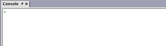
Deephaven is now ready for use.
Step 2 - Access Your Data
Deephaven uses data stored in tables. These tables are organized by namespaces. This is analogous to the way you store information on your computer. Just as you might use folders (or directories) to hold individual files, Deephaven uses namespaces to hold individual tables.
To access tables in Deephaven, you need to know:
- where the table is located (the name of the namespace), and
- the name of the table
For this exercise we are going to access the namespace called LearnDeephaven, and open a table called StockTrades. (Note: This configuration should be included with the default Deephaven installation. Contact your system administrator if it is not.)
You also need to know how to write the instructions to tell Deephaven what to do. These instructions are called queries, and they are written using the Deephaven Query Language.
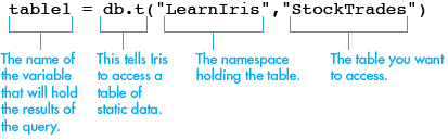
Write Your First Query
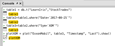
Click your mouse anywhere in the Console panel and type the following:
table1 = db.t("LearnDeephaven","StockTrades")
This is a Deephaven query. More details about the Deephaven Query Language is included in the documentation, but the following diagram summarizes what the query is asking Deephaven to do:
Press Enter or Return on your keyboard to run the query in Deephaven.
A new tabbed panel named table1 is added to the lower part of the Deephaven console, as shown below.
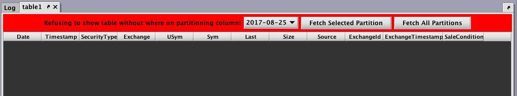
The table you just accessed is partitioned. In a nutshell, this means the table is organized and grouped into different smaller segments. By organizing a table like this, the computing power needed for analysis can be applied more efficiently, especially when your table has millions or billions of rows of data. In this case, the table is partitioned by the date shown in the first column.
For this exercise, go ahead and click Fetch Selected Partition.
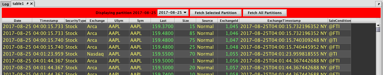
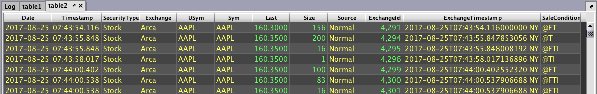
The panel will now fill in with a table that holds 12 columns including Date, Timestamp, SecurityType, Exchange, USym, Sym, Last, Size, Source, ExchangeId, ExchangeTimestamp and SaleCondition.
Congratulations! You have just run your first query! Using the Deephaven console, you accessed a table stored in a namespace, and then stored the contents of that table to a new table named table1.
Step 3 - Manipulate the Data
Now that we have a table loaded into the Deephaven console, we can further manipulate the data to serve our needs. For example, we can filter the data to include only certain categories, values or other aspects. We can add new columns or remove columns we don't need. Or, we can sort, group or aggregate the data, or join the data in this table with data from another table. The Deephaven Query Language provides many methods for manipulating the data further. However, since we are just getting started, we will stick with something relatively simple.
Filtering Data
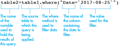
The table now holds quantitative information about the individual trades for each of 10 different financial securities (AAPL, AXP, BAC, CSCO, GOOG, IBM, INTC, MSFT, PFE, XOM). If you scroll in the window holding the table, you can start to get a sense of the large volume of data the table holds. However, we can eliminate unwanted data by filtering out the information we do not want. This is done using the where() method in Deephaven. Here's the new query:
table2=table1.where("Date=`2017-08-25`")
The following diagram summarizes the components of this query:
Copy the query above and then paste it into the Deephaven Console window (or retype it if you prefer). Then press Enter on your keyboard.
When this query runs in Deephaven, a new tab for table2 appears in the lower part of the console window. The red "partition" banner is no longer on the table because you just filtered the table to a specific date partition. Specifically, you filtered the table to show only the data for August 25, 2017.
Let's run another filter. This time we'll use the where method to filter the table to include only one of the ten ticker symbols in the table.
Here's the query:
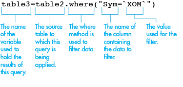
table3=table2.where("Sym=`XOM`")
This is very similar to the last query, but this time we are filtering on the XOM value, which is a value in the column named Sym. The following diagram summarizes the components of this query:
Copy the query above and then paste it into the Deephaven Console window (or retype it if you prefer). Then press Enter on your keyboard.
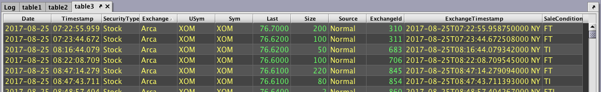
When this query is run in Deephaven, a new tab for table3 appears in the lower part of the console window. If you scroll through the table, you'll see it only contains the data for when the value XOM is contained in the column titled Sym. The data has now been reduced to only 38,387 rows.
Step 4 - Make a Plot
In the previous step, we filtered the table to show (a) only one day's worth of data for (b) only one ticker symbol from the Sym column. We can now plot that data to more easily visualize any trend or pattern it may show. Here's the query to plot the price of that ticker symbol over the course of that one day:
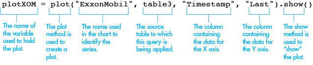
plotXOM = plot("ExxonMobil", table3, "Timestamp", "Last").show()
The following diagram summarizes the components of this query:
Copy the query above and then paste it into the Deephaven Console window (or retype it if you prefer). Then press Enter on your keyboard.
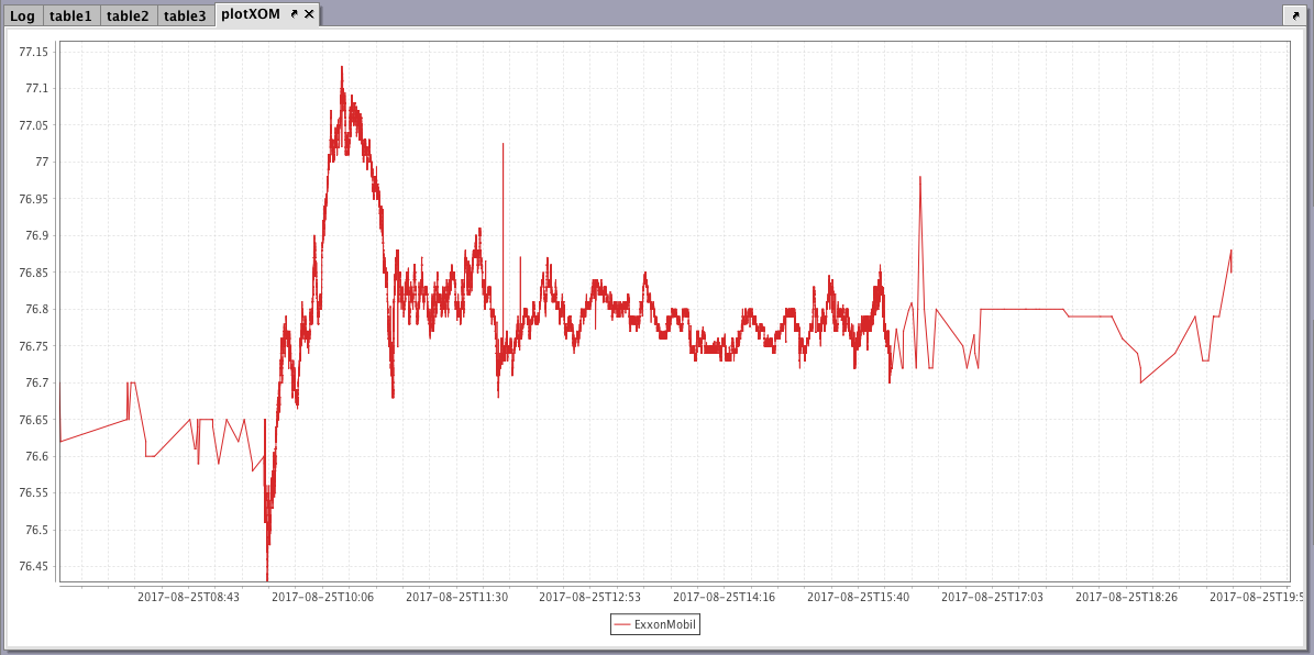
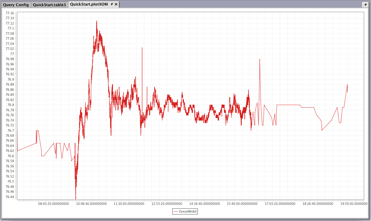
After this query runs in Deephaven, a new panel titled plotXOM appears in the lower part of the console window. This panel shows a plot that charts the variation in the price of ExxonMobil stock over the course of one day.
Congratulations! You just used Deephaven to make your first plot.
Step 5 - Create and Save a Persistent Query
So far, you've accessed data, filtered the data, saved the data and made a plot. You've completed those steps by using queries in the Deephaven console. What if you wanted to save those queries so you could use them later. Or maybe you want to share those queries or the tables generated by the queries with other individuals or teams within your enterprise. If any of those scenarios apply, you should consider making your query persistent - meaning the query is saved and stored. Let's see how to create a persistent query.
First, highlight all of the content that you currently have in the Console panel, and then copy that content to your clipboard. [Right-click > Copy; or Ctl+C (Windows); or ⌘+C (MacOS)]
It should look something like the following before you highlight the content:
After copying the content, click the Query Config button at the top of the interface. A dialog window will then present the option to rename the panel, or keep the existing Query Config name.
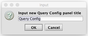
Click OK to keep the same name.
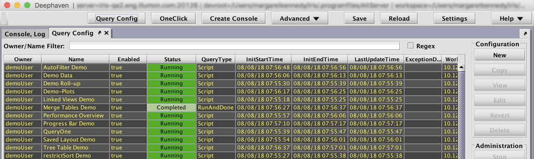
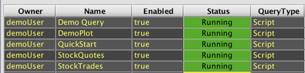
Deephaven will then connect to the server and present a new window called the Query Config window. This window shows the names and some of the properties associated with persistent queries that have already been created and saved to Deephaven by someone in your enterprise, as demonstrated below.
Click the New button, which can be found in the Configuration section in top right corner of this panel. This will open the Persistent Query Configuration Editor window.
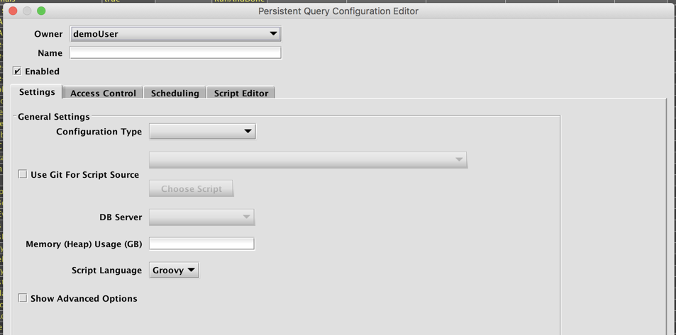
In the Name field, enter the name you would like to use for this query. (e.g., QuickStart)
In the drop-down menu to the right of Configuration Type, select Live Query (Script).
In the drop-down menu to the right of DB Server, select the first option available. (Server names vary by customer.)
In the field to the right of Memory (Heap) Usage, enter the number 4. (This is the amount of RAM that will be assigned to run your persistent query.)
Then, select the tab titled, Script Editor. This will open a new blank panel.
Click your mouse anywhere inside the Script Editor panel, and paste the content previously copied from the Console window.
The Script Editor window should now look very similar to the following:
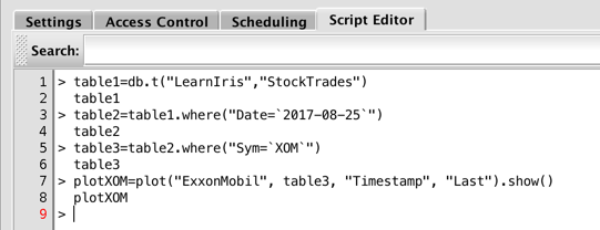
We need to do a little clean-up to remove some artifacts copied from the console. At the beginning of each line is the greater-than symbol (>) and a space. Remove them from each line. Also, between each of the longer lines is the name of the table (or plot) the previous line generated. Remove those values as well.
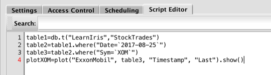
The contents in the Script Editor window should now look like this:
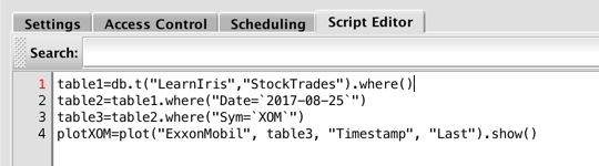
In order for each table to open properly when the persistent query runs, we need to update the script ine line 1 for table1. When we attempted to open this table in the console, we were asked to fetch a selected partition, or to open all partitions. If we want all the partitions in table1 to open without filtering to a specific date, as in table2, we can add an empty .where() filter to or query, as shown below:
Click the OK button at the bottom of the window. Doing this will save your persistent query and return you to the Query Config window. Your newly created persistent query should be listed in alphabetical order. In the Status column, the value in the row for the QuickStart query should show values changing from Acquiring Worker to Initializing to Running.
Congratulations! You have now saved your first persistent query. Now we can demonstrate how persistent queries work.
Start by quitting the Deephaven application. (Ctrl+Q: Windows; ⌘+Q: macOS). You'll be asked if you want to save your workspace. Click No. Then, restart Deephaven using the same process used earlier (before you started this Quick Start Guide.)
When Deephaven restarts, you should see the same empty console you saw earlier.
Click Query Config at the top of the Deephaven interface. As before, a dialog window will present the option to rename the panel, or keep the existing Query Config name. Click OK to keep the same name. Deephaven will then connect to the server and present Query Config panel.
The QuickStart query you just saved should now be listed in alphabetical order in the panel. Because you saved this as a persistent query, you can now also retrieve each of the three tables and the plot you were created earlier – all without having to retype the queries.
To open a table associated with the QuickStart query, first highlight the row in the QueryConfig panel that contains the QuickStart query. At the bottom of the Deephaven interface, you'll see the button Show Table. To the right of that button is a drop-down menu. Click the drop-down menu and select table3 as shown below.
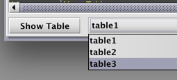
Then click Show Table.
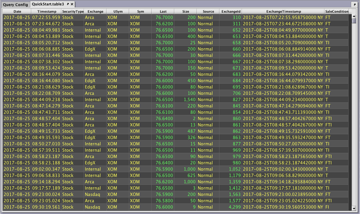
A new panel opens in the Deephaven console with a tab named QuickStart.table3, as shown below.
You can also open a plot in a similar fashion. We first need to return to the list of persistent queries, so click the tab labeled Query Config at the top left portion of the console window. Then, just as you did before, click once on the row containing the QuickStart query.
At the bottom of the Deephaven interface, you'll see the button Show Widget. (Note: "Widget" is a term used to describe various user interface components. In Deephaven, a plot is a common form of widget.)
To the right of the Show Widget button is a drop-down menu. Click the drop-down menu and select plotXOM, as shown below. There is only one plot associated with this query, so there is only one option in the drop-down menu. If the query generated more than one plot, the names of all of the generated plots would be in this list.
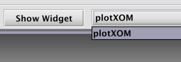
Then click Show Widget.
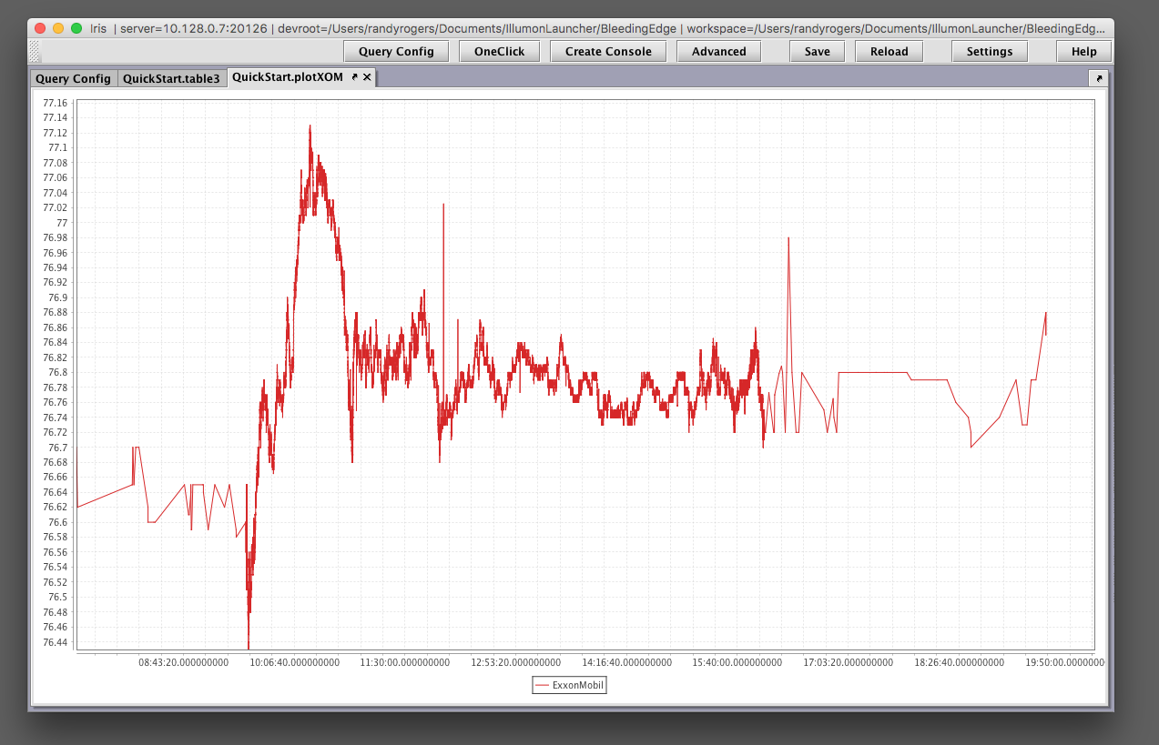
A new panel opens in the Deephaven console with a tab named QuickStart.plotXOM, as shown below.
Congratulations! You just opened a table and a plot created by a persistent query.
Step 6 - Customize Your Workspace
The Deephaven interface is designed to be modular so you can build your own customized workspace. Let's take a look.
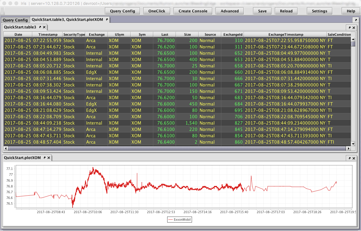
If you've completed the previous five steps, your Deephaven console window should have three panel tabs showing. In order from left to right, the tabs should be QueryConfig, QuickStart.table3 and QuickStart.plotXOM, as shown below
The default order of the tabs shown are the same as the order in which they were built (or revealed) However, the default layout is easy to change.
Each panel in the interface has a tab, which contains the name of the panel. And, each panel can be moved to a different part of the interface by clicking, holding and dragging the tab with your mouse.
Click the tab titled, QuickStart.table3 to bring it to the front.
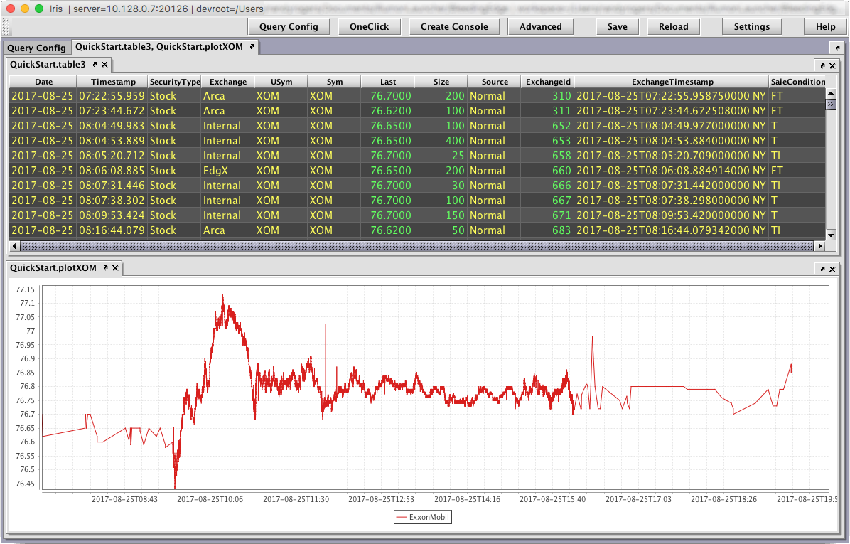
Hover your mouse cursor over the tab titled, QuickStart.plotXOM. Click and hold down the mouse button. While holding down the mouse button, "drag" the panel until its tab is positioned in the lower half of the panel containing QuickStart.table3. Thick black lines will show you how the panel will be positioned when you release the mouse. When the black lines show placement in the lower portion of the plotX panel, release the mouse button. The two panels should now be nested together in one common panel titled QuickStart.table3,QuickStartplotXOM.
The plot only takes up about one third of the vertical space in the panel; however, you can resize the panel containing the plot. When you place your mouse cursor near the horizontal border at the bottom of the table, the cursor will change to the "row resize" shape ( ), which allows you to adjust the border vertically. You can then click, hold and drag the border between the two panels up or down to adjust the height of the panel.
In the following example, the panel containing the plot has been enlarged.
Congratulations! You've just built and customized your first workspace. Click the Save button at the top of the Deephaven interface to save your new workspace.
To learn more about using Deephaven for big data analyses, please refer to the Deephaven Documentation Website.
Last Updated: 28 February 2020 12:20 -05:00 UTC Deephaven v.1.20200121 (See other versions)
Deephaven Documentation Copyright 2016-2020 Deephaven Data Labs, LLC All Rights Reserved